![[논문 리뷰] Prioritized Generative Replay](/assets/img/251002/thumbnail.png)
[논문 리뷰] Prioritized Generative Replay
작성자: 이동진
논문 정보
제목: Prioritized Generative Replay
저자: Renhao Wang, Kevin Frans, Pieter Abbeel, Sergey Levine, Alexei A. Efros, UC Berkeley.
학회: ICLR 2025
Overview
- Target task: Off-policy learning, Sample efficient, DMC-100K
- Algorithm class: SAC (state-based tasks), DrQ-v2 (pixel-based tasks)
- Motivation
- Distribution of states an agent visits is different from the optimal distribution of states the agent should train on.
- Certain classes of transitions are more relevant to learning, i.e. data at critical decision boundaries or data that the agent has seen less frequently.
- Solution: Conditional Diffusion Model
- Densification of past experience: Generative models 사용하자
- Guidance towards useful experience: Priority에 따라 샘플링할 수 있어야 한다.
Background
Reinforcement Learning (논문에서 자주 쓰이는 표기들만 정리)
- $\tau = (s, a, r, s’)$
- $\mathcal{D}$: a finite replay buffer of transitions
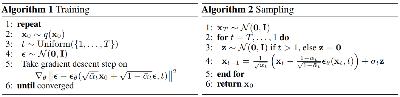
Diffusion Models
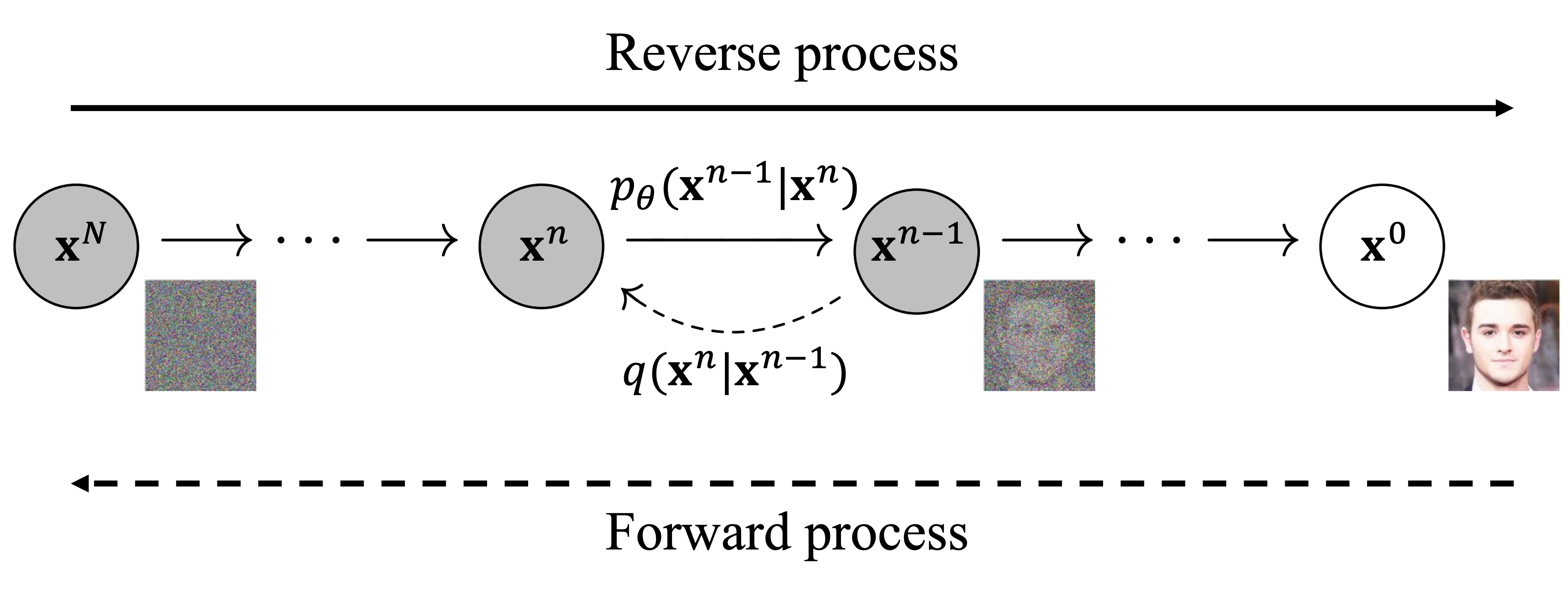
- Diffusion model의 컨셉은 데이터 $\mathbf{x}^0 \sim p_{\text{data}}(\mathbf{x})$와 가우시안 노이즈 $\mathbf{x}^{N} \sim \mathcal{N}(\mathbf{0}, I)$ 사이를 실제로 $N=128$ steps 동안 노이즈를 추가하거나 제거하며 왔다 갔다 하는 과정이 있을 것 같지만, 학습 동안에는 한 step에 사용된 노이즈를 예측하는 방식으로 네트워크가 학습됨
-
모든 데이터 $\mathbf{x}^0$와 모든 $n=1,\ldots,128$에 대해서, $\mathbf{x}^{n}$에서 걷어내야 할 노이즈 $\bm{\epsilon}$를 예측하는 네트워크 $\bm{\epsilon}_\theta(\mathbf{x}^{n}, n)$를 학습
\[\operatorname*{\mathbb{E}}\limits_{\substack{\mathbf{x}^{0}\sim p_{\text{data}}\\ n\sim\text{Unif}(\{1,\ldots,N\})\\ \bm{\epsilon}\sim\mathcal{N}(\mathbf{0},I)}} \left[ \lVert \bm{\epsilon} - \bm\epsilon_\theta(\mathbf{x}^n,n) \rVert_2^2\right],\]where $\mathbf{x}^{n}=\sqrt{\bar{\alpha}_t}\mathbf{x}^{0} + \sqrt{(1-\bar{\alpha}_t)}\bm{\epsilon}$. (forward pass를 직접 해서 $\mathbf{x}^{n}$을 만드는 것이 아니라 그것과 동치인 closed form이 있음)
Classifier-Free Guidance (CFG)
- 각 데이터 $\mathbf{x}^{0}\in p_{\text{data}}$마다 그것과 관련된 condition $c$ (e.g., class, attribute, label 등)에 접근할 수 있다면,
-
즉, 데이터셋 구성이 $(\mathbf{x}, c)$이라면 diffusion models을 conditional diffusion model로 확장시킬 수 있음
\[\operatorname*{\mathbb{E}}\limits_{\substack{(\mathbf{x}^{0}, c)\sim p_{\text{data}}(\mathbf{x},c)\\ n\sim\text{Unif}(\{1,\ldots,N\})\\ \bm{\epsilon}\sim\mathcal{N}(\mathbf{0},I) \\p \sim \text{Bernoulli}(p_{\text{uncond}})}} \left[ \lVert \bm{\epsilon} - \bm\epsilon_\theta(\mathbf{x}^n,n,(1-p)\cdot c+p\cdot\varnothing) \rVert_2^2\right].\]where $p_{\text{uncond}}$ is a hyperparameter.
-
샘플링시 걷어낼 최종 노이즈는 다음과 같이 사용
\[\tilde{\bm{\epsilon}}_\theta(\mathbf{x}^n, n, c)=\omega\cdot \bm\epsilon_\theta(\mathbf{x}^{n},n,c) + (1-\omega)\cdot\bm{\epsilon}_\theta(\mathbf{x}^n,n,\varnothing),\]where $\omega$ is a hyperparameter, called the guidance scale.
Method: Prioritized Generative Replay (PGR)
Key Points of Algorithm
- Replay buffer $\mathcal{D}_{\text{real}}$을 conditional diffusion model $G(\tau \mid c)$을 사용하여 학습할 것이다.
- $G$에 condition $c$를 줘서 condition과 relevant한 sample을 생성할 것이다.
- 이때, condition $c$ 값에 큰 priority 값을 줘서 높은 priority를 갖는 transition $\tau$를 생성할 것이다.
- 각 transition $\tau=(s,a,r,s’)$에 priority를 주는 함수를 relevance function $\mathcal{F}(\tau)$ 라고 부를 것이다.
- 알고리즘
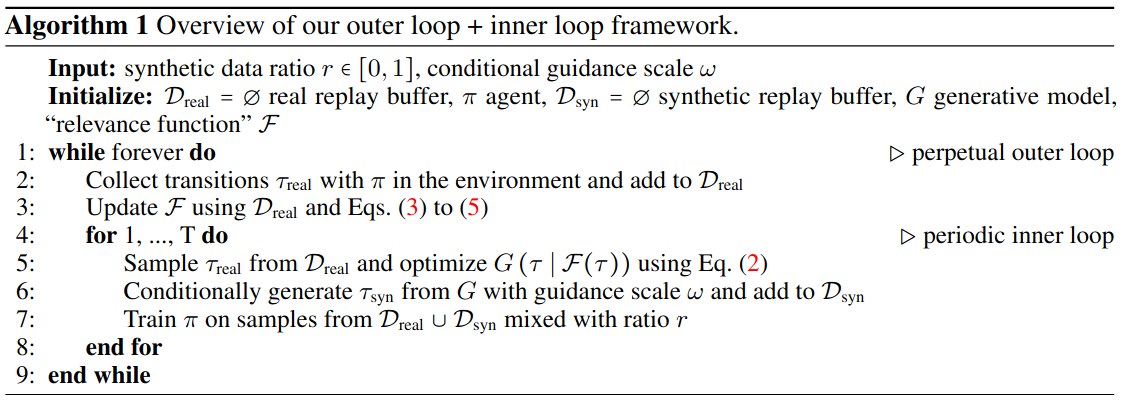
- 5. Diffusion 학습: $\mathcal{D}_{\text{real}}$ 안의 모든 $\tau$에 대해서 $\mathcal{F}(\tau)$을 계산하고, 그 중 상위 $5\%$ transition-condition pair $(\tau, \mathcal{F}(\tau))$로 conditional diffusion model $G(\tau \mid \mathcal{F}(\tau))$ 학습. 이때, $p_{\text{uncond}}=25\%$의 확률로 uncondition으로 바꿔줌.
- 6. 데이터 생성: 위에서 만들어 놓은 상위 $5\%$의 $\mathcal{F}(\tau)$을 condition으로 줘서 인위 데이터를 1M개 생성하고 $\mathcal{D}_{\text{syn}}$에 저장 ($\mid \mathcal{D}_{\text{syn}} \mid=1\text{M}$).
- 7. Off-policy 학습 총 batch size 256 중 $r=50\%$ 는 $\mathcal{D}_{\text{real}}$에서 나머지는 $\mathcal{D}_{\text{syn}}$에서 샘플링하여 off-policy learning 수행
Relevance Functions
좋은 relevance function이 되기 위한 2가지 요건 (desiderata)
- 계산량이 적어야 한다.
- 쉽게 overfitting이 되면 안 된다 ($c$값도 다양해야 하고, 같은 $c$값에 대해서 $\tau$도 다양해야 한다.)
Relevance function 예시들
- Ex 1) Return: $\mathcal{F}(s,a,r,s’)=Q(s, \pi(s))$
- On-policy sample들을 더 많이 뽑게 만들어 준다.
- High-return transitions들의 다양성이 적기 때문에 과적합 위험이 있다.
- Ex 2) TD error: $\mathcal{F}(s,a,r,s’)=r+\gamma Q(s’, \pi(s’))-Q(s,a)$
- Critic network가 o.o.d에 정확성이 낮기 때문에 $\mathcal{F}$의 정확성도 떨어지게 된다.
- Ex 3) Curiosity: $\mathcal{F}(s,a,r,s’)=\frac{1}{2}\lVert g(h(s),a)-h(s’) \rVert^2$
- $h(s)$: Encoder
- $g(s, a)$: Forward dynamics model
- 제일 좋음
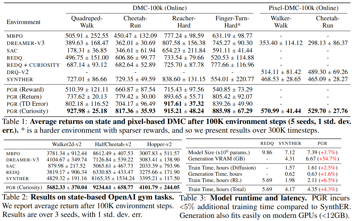
Experiment
환경: DMC, OpenAI gym 둘 다 100K 상호작용
Ablation.
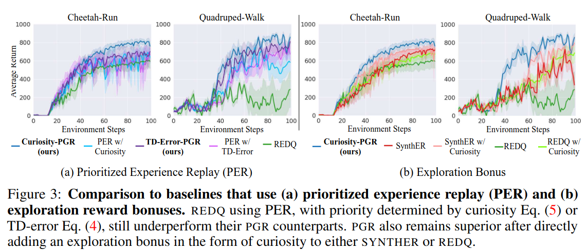
- (a) Generative replay의 중요성: Prioritized generative replay vs. prioritized experience replay
- (b) Conditioning의 중요성: Prioritized generative replay vs. SynthER (+ 단순 exploration bonus)
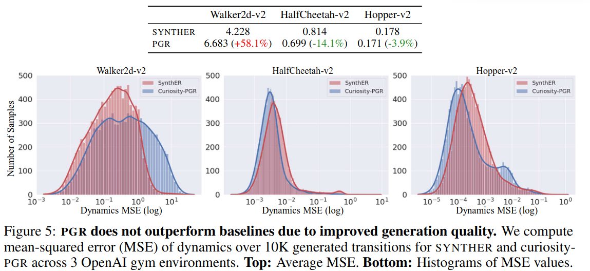
- PGR이 SYNTHER보다 생성한 데이터 퀄리티 (faithfulness)가 더 좋아서 성능이 좋아진 것이 아니다.
- Dynamics MSE:
- 생성한 $\hat{\tau}=(\hat{s}, \hat{a}, \hat{r}, \hat{s}’)$에 대하여,
- 환경을 $\hat{s}$으로 reset 시키고 $\hat{a}$를 수행하여 실제 $r$ 과 $s’$ 획득
- $MSE(r, \hat{r}), MSE(s’, \hat{s}’)$ 계산
Reduction in overfitting
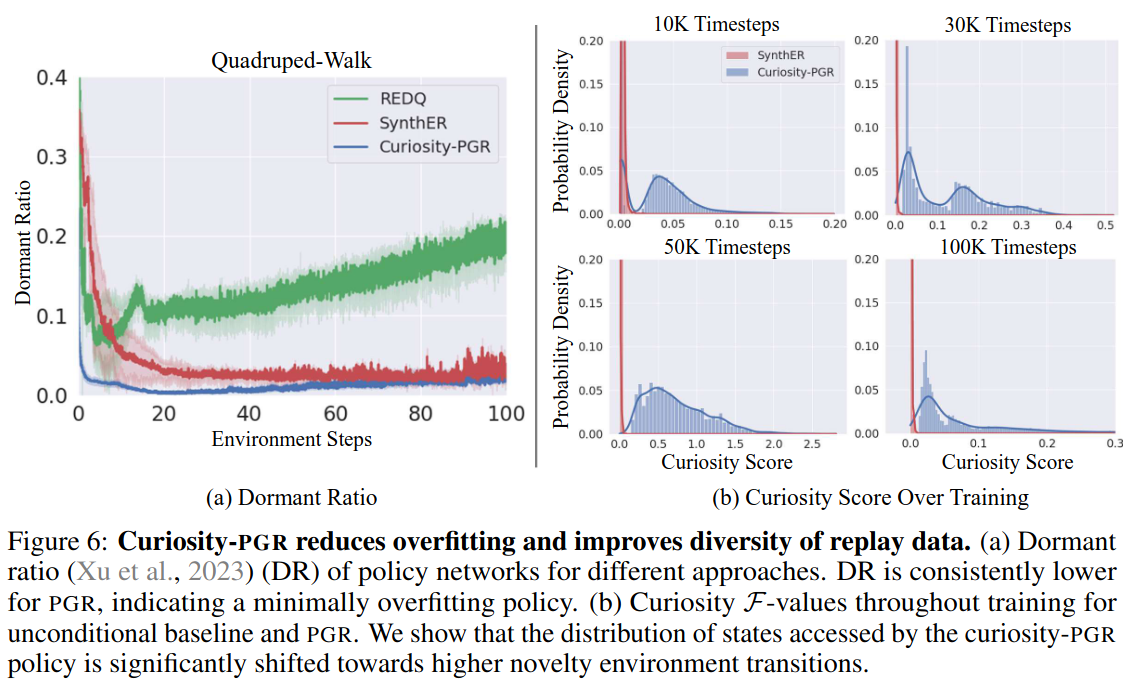
(a) Dormant Ratio: 네트워크 안에서 대부분의 데이터에 대해서 activation이 0인 뉴런의 비율. 주로 overfitting이 발생했거나 biased된 네트워크는 dormant ratio가 높음.
(b) 학습에 따른 데이터의 Curiosity의 분포도 ⇒ 데이터의 다양성을 보여줌
Scaling behavior
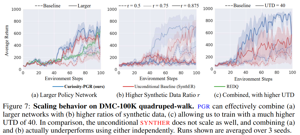
- (a) 네트워크 사이즈를 늘리거나, (b) synthetic data에 더 의존하거나, (c) Update-to-Data (UTD)를 늘렸을 때, PGR이 효과가 크다.