![[논문 리뷰] Towards General-Purpose Model-Free Reinforcement Learning](/assets/img/250508/image_6.png)
[논문 리뷰] Towards General-Purpose Model-Free Reinforcement Learning
작성자: 이동진
논문 정보
제목: Towards General-Purpose Model-Free Reinforcement Learning
저자: Scott Fujimoto, Pierluca D’Oro, Amy Zhang, Yuandong Tian, Michael Rabbat, Meta FAIR.
학회: ICLR 2025
Overview
- Target task: Online model-free RL
- Algorithm class: Off-policy learning, TD3 계열 (deterministic actor, double critic), Representation learning
- Motivation
- Model-free RL 알고리즘들은 문제 상황마다 domain-specific하게 개발되어 왔다.
- e.g., DQN for a discrete action space, DDPG for a continuous action space, DrQ for a pixel observation space, …
- Dreamer-v3, TD-MPC2 등 model-based RL이 벤치마킹 가리지 않고 높은 성능을 보일 수 있는 이유는 MDP 모델 학습 중 representations 덕분일 것이다.
- Model-free RL 알고리즘들은 문제 상황마다 domain-specific하게 개발되어 왔다.
- Solution
- Model-based objective를 사용하는 representation learning을 추가
- 구현 디테일을 추가하여 discrete action space에도 사용할 수 있는 TD3를 만들자
Introduction
강화학습 이론 자체는 MDP에 대한 특별한 가정 없이 기술되어 있지만, 구현체들은 문제 상황마다 서로 다른 domain-specific한 알고리즘들이 고안되어 왔다.
- ex1) Discrete action vs. continuous action (DQN vs. DDPG)
- Q-learning 이론 자체는 discrete/continuous action 상관 없이 기술할 수 있지만 continuous action의 경우 max 값을 구하기 어려워서 deterministic policy gradient를 사용하거나 SAC처럼 reparametrization을 사용한다
- ex2) Vector observation vs. pixel observation (SAC vs DrQ)
- SAC에 CNN policy를 달아도 representation learning 없이는 학습이 거의 안 된다.
- DrQ는 representation learning 없이도 pixel observation으로부터 잘 학습하는 알고리즘이지만 vector observation에는 사용할 수 없다.
- ex3) Specialized to a specific environment (AlphaGo for Go)
❓ 지금까지의 general-purpose RL 알고리즘
- Model-free 알고리즘
- 예시: PPO 등 on-policy policy gradient 방법론들
- 장점: MDP에 대해서 특별한 가정을 하지 않기 때문에 범용적으로 사용됨.
- 단점: On-policy learning이기 때문에 sample inefficient하고 local minima에 빠지기 쉽다 (why?).
- Model-based 알고리즘
- 예시: Dreamer-v3, TD-MPC2 등
- 장점: a single hyperparameter setting으로 여러 벤치마킹 환경에서 좋은 성능 기록
- 단점: 시간 및 계산 복잡도가 높다. (e.g., large network, simulated rollout, planning)
💡 MR.Q의 motivation
가정: Model-based 알고리즘의 높은 성능은 MDP 모델 학습 중 implicit하게 학습되는 representations 덕분일 것이다.
주장: Model-based objective을 사용하는 representation learning을 추가한다면, simulated rollout / planning 없이 model-free RL의 성능을 개선할 수 있을 것이다.
✏️ Comments
- 이 논문은 general-purpose RL 알고리즘을 고안하는 것보다는 representation learning 방법론을 고안하는 논문에 더 가깝다.
- 지금까지는 image observation에 대해서만 representation learning 해왔지만, 저자의 이전 논문 TD7 [1]에서는 vector observation에 대해서도 representation learning하는 것이 좋다고 주장하고 있다.
Model-Based Representations For Q-Learning (MR.Q)
Notations \(\begin{align} f_\omega:s \mapsto \mathbf{z}_s, & \quad\quad\quad g_\omega : (s,a) \mapsto \mathbf{z}_{sa},\\\ \pi_\phi: \mathbf{z}_s \mapsto a, & \quad\quad\quad Q_\theta:\mathbf{z}_{sa} \mapsto q. \end{align}\)
- Implementations에서는 $\mathbf{z}_s, \mathbf{z}_{sa} \in \mathbb{R}^{512}.$
흔히 사용되는 representation learning objective
-
Dynamics learning에서 motivation을 얻어서 $(s, a)$에 대한 임베딩 $\mathbf{z}_{sa}$가 $s’$ 에 대한 임베딩 $\mathbf{z_{s’}}$에 가까워지도록 학습
\[\mathcal{L}(\omega) =\left( g_\omega ( f_\omega(s),\,a) - \mid f_\omega(s') \mid_\times \right)^2 = \left( \mathbf{z}\_{sa} - \mid \mathbf{z}\_{s'}\mid_\times\right)^2.\] - Issue: $g_\omega$가 dynamics model in a latent space의 역할을 하게 되는데, 우리의 목적은 representation learning이지 dynamics model을 학습하는 것이 아님
- Solution: Linear MDPs 분야에서 영감을 받아서 임베딩 벡터 $\mathbf{z}_{sa}$를 선형변환한 $\mathbf{z}_{sa}^\top W_p$를 $\mathbf{z_{s’}}$에 가까워 지도록 하자.
Theoretical Motivation from Linear MDPs
Linear MDPs 분야에서는 state-action 임베딩 벡터 $\mathbf{z}_{sa}$와 true action value $Q^{\pi}(s,a)$가 approximately 선형 관계가 있다고 가정하고 다음과 같이 근사
\[Q(s,a)=\mathbf{z}_{sa}^\top \mathbf{w}.\]
Linear MDPs 분야에서 feature selection 방법 (최적의 $\mathbf{w}$ 찾는 방법)
-
Model-free 방법 ⇒ Bellman equation 사용
\[\mathbf{w} \leftarrow \mathbf{w} - \alpha \mathbb{E}_D\left[ \nabla_\mathbf{w} \left( \mathbf{z}_{sa}^\top \mathbf{w} - \mid r+\gamma\mathbf{z}_{s'a'}^{\top}\mathbf{w} \mid_\times\right)^2\right],\]where $D=\lbrace (s, a,r,s’,a’) \rbrace$.
-
Model-based 방법
\[\begin{align*} & \mathbf{w}_r := \operatorname*{argmin}_\mathbf{w} \mathbb{E}_D \left[ \left(\mathbf{z}_{sa}^\top\mathbf{w} - r \right)^2\right], & \quad\quad W_p:= \operatorname*{argmin}_W \mathbb{E}_D \left[ \left(\mathbf{z}_{sa}^\top W - \mathbf{z}_{s'a'} \right)^2\right], \\ &\mathbf{w}_{\text{mb}} := \sum_{t=0}^{\infty} \gamma^{t} W_p^t \mathbf{w}_r. \end{align*}\]- $\mathbf{z}_{sa}^\top\mathbf{w}_r$이 estimated reward model
- $\mathbf{z}_{sa}^\top W_p$가 estimated dynamics model
- 엄밀히 말하면, 학습 target이 $\mathbf{z}_{s’a’}$이기 때문에 다음 상태 뿐만 아니라 $a’$까지 정책 dependent한 dynamics model로 해석됨
- 진짜 dynamics model을 학습하기 위한 것이 아닌 $\mathbf{z}_{sa}^\top \mathbf{w} \approx Q^{\color{red}{\pi}}(s, a)$이길 바라기 때문
이렇게 찾은 $\mathbf{w}$ 또는 $\mathbf{w}_{\text{mb}}$에 대한 이론

- 내용: 수렴 지점에서 $\mathbf{w} = \mathbf{w}_{\text{mb}}$다 (이 논문에서는 중요하지 않음).
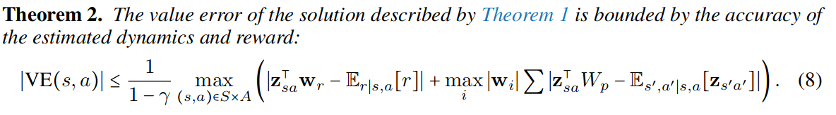
- 내용: Value error $\text{VE}(s, a)=Q(s,a)-Q^{\pi}(s, a)$가 estimated reward and dynamics models의 정확도에 bound된다.
- 즉, Model이 정확할수록 $\mathbf{z}_{sa}^\top \mathbf{w}_{\text{mb}}$ 가 true action value function에 가까워진다.
최종적으로 다음과 같은 representation learning objective를 생각해볼 수 있다.
하지만 $\mathbf{z}_{s’a’}$에서 $a’$이 거슬리기 때문에 MR.Q에서는 다음과 같이 완화된 objective를 제안
\[\mathcal{L}(\mathbf{z}_{sa}, \mathbf{w}_r, W_p)= \mathbb{E}_D \left[ \left(\mathbf{z}_{sa}^\top\mathbf{w}_r - r \right)^2\right] + \lambda \mathbb{E}_D \left[ \left(\mathbf{z}_{sa}^\top W_p - \bar{\mathbf{z}}_{s'} \right)^2\right],\]where $\bar{\mathbf{z}}_{s’} = f_{\bar{\omega}}(s’)$ is provided by target encoder network.
완화된 버전을 사용할 경우 Theorem 2 ($\mathbf{z}_{sa}^\top \mathbf{w} \approx Q^{\pi}(s, a)$)이 더 이상 보장되지 않지만, $\mathbf{z}_{sa}$이 충분히 rich할 경우 $\hat{Q}(\mathbf{z}_{sa}) = Q^{\pi}(s, a)$을 만족하는 어떤 비선형 함수 $\hat{Q}$가 존재한다 (⇒ Theorem 3)
Algorithm
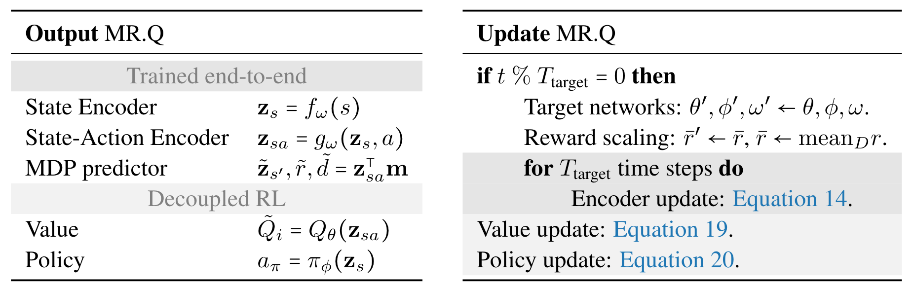
- 알고리즘 뼈대: TD3에 encoders $f_\omega(s), g_\omega(\mathbf{z}_s, a)$가 추가된 버전.
- MLP predictor $\mathbf{m}$: 벡터가 아닌 행렬이고, $\mathbf{z}_{sa}$로부터 다음 상태 벡터 $\mathbf{z}_{s’}$, 보상 $r$, done boolen $d$ 를 예측하는 역할
- 더 자세히는 $\mathbf{m}$ = nn.Linear($d_{\text{latent}}$, $d_{\text{latent}}$ + $N_{\text{bins}}$ + 1)
1. Encoder 학습
- Encoders 학습은 매 $T_{\text{target}}=250$ (target networks 업데이트 주기)마다 발생
- 1-step transition $(s,a,r,d,s’)$을 사용하지 않고, 길이 $H_{\text{enc}}$의 subtrajectory $(s_0, a_0, r_1, d_1, s_1, \ldots, R_{H_{\text{enc}}}, d_{H_{\text{enc}}}, s_{H_{\text{enc}}})$를 사용하여 중간 결과물들도 함께 매칭시켜 줌.
-
즉, 다음과 같이 unrolling of the learned dynamics model 수행
\[\tilde{\mathbf{z}}_s^t, \tilde{r}^t, \tilde{d}^t=g(\tilde{\mathbf{z}}_s^{t-1}, a^{t-1})^\top \mathbf{m}, \quad \quad \tilde{\mathbf{z}}_s^0 = f_\omega(s_0).\]
-
그리고 다음과 같이 손실함수를 구성

- $\mathcal{L}_{\text{Reward}}(r, \tilde{r}):=\text{CE}(\tilde{r}, \text{Two-Hot}(r)).$
- Two-Hot 예시: 보상 범위 $[-10, 10]$을 $N_{\text{bins}}=20$ 구간으로 나눴다고 했을 때, $r=5.1$에 대해서는 왼쪽 차원에는 0.1, 오른쪽 차원에는 0.9를 할당하는 방법
- $\mathcal{L}_{\text{Dynamics}}(\mathbf{z}_s, \tilde{\mathbf{z}}_s):=\left( \tilde{\mathbf{z}}_s - \mathbf{z}_s\right)^2.$
- $\mathcal{L}_{\text{Terminal}}(d, \tilde{d}):=( \tilde{d} - d)^2.$
- $\mathcal{L}_{\text{Reward}}(r, \tilde{r}):=\text{CE}(\tilde{r}, \text{Two-Hot}(r)).$
2. Policy 학습
-
TD3 정책 학습 방법
\[\mathcal{L}(\phi)=- 0.5 \sum_{i=\{ 1, 2\}} Q_{\theta_i} ( s,\pi_\phi(s) ).\] -
MR.Q 정책 학습 방법
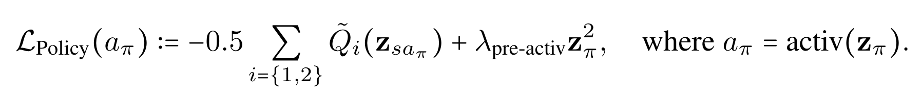
where $\mathbf{z}_{\pi}$는 actor network의 pre-activation output.
- Continuous action일 경우 ⇒ tanh 사용 ⇒ 그냥 TD3처럼
- Discrete action일 경우 ⇒ Gumble softmax를 통해 reparametrization
3. Critic 학습
-
TD3 Critic 학습 방법: transition $(s, a, r, s’)$에 대하여
\[\mathcal{L}({\theta_i})=\left(r+\gamma \operatorname*{min}_{j=\{ 1,2 \}}Q_{\bar{\theta}_i}(s', a'_{\pi}) - Q_{\theta_i}(s, a)\right)^2,\]where $a’_{\pi} = \text{clip}(\pi_{\bar{\phi}}(s’) + \bar{\epsilon}, -1, 1)$ for $\bar{\epsilon} = \text{clip} (\epsilon, -c, c)$ and $\epsilon \sim \mathcal{N}(0,1)$ (target policy smoothing)
-
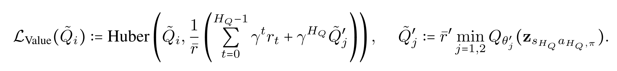
MR.Q Critic 학습 방법: $n$-step transition $(s_t, a_t, \sum\limits_{k=0}^{n-1}\gamma^{k} r_{t+k}, s_{t+n})$에 대하여 ($n=3$)
\[\mathcal{L}({\theta_i})=\text{Huber}\left( Q_{\theta_i}(\mathbf{z}_{sa}^t), \sum\limits_{k=0}^{n-1}\gamma^{k} r_{t+k} + \operatorname*{min}_{j=\lbrace1, 2\rbrace} Q_{\bar{\theta}_i}(\mathbf{z}_{sa_\pi}^{t+n}) \right).\]where
\[a_\pi^{t+n}=\begin{cases}\displaystyle\operatorname*{argmax} a' & \text{for discrete }\mathcal{A}, \\ \text{clip}(a', -1 ,1) & \text{for continuous }\mathcal{A}, \end{cases}\]for
\[a'=\pi_{\bar{\phi}}(\mathbf{z}^{t+n}_s)+\text{clip}(\epsilon,-c,c), \text{ and } \epsilon \sim \mathcal{N}(0,1).\]
그 외 구현 디테일
- Replay buffer로 LAP [2] 사용
-
Critic 업데이트에서 TD target을 $\bar{r}$로 scaling 해줌
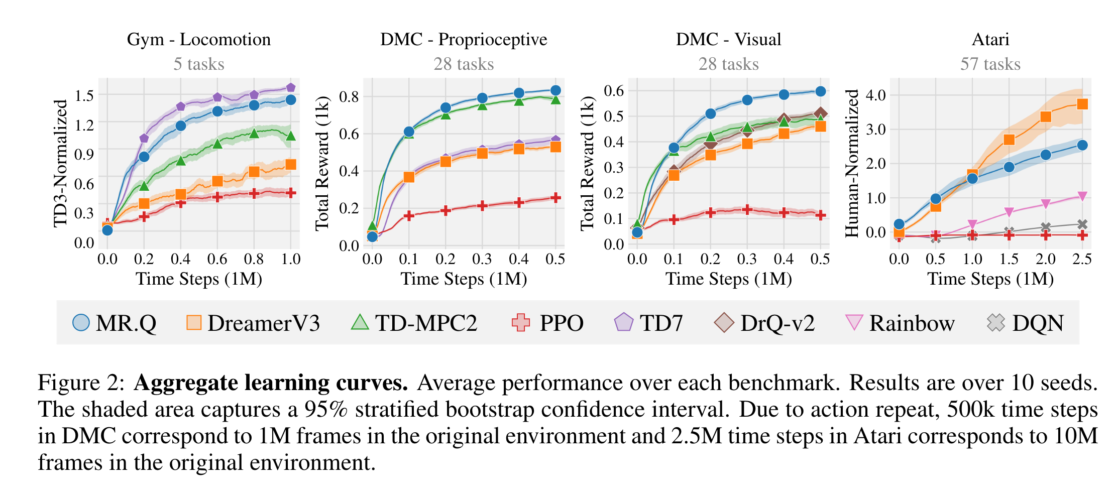
Experiment
Reference
[1] Fujimoto, Scott, et al. “For sale: State-action representation learning for deep reinforcement learning.” Advances in neural information processing systems, 36 (2023)
[2] Fujimoto, Scott, et al. “An equivalence between loss functions and nonuniform sampling in experience replay.” Advances in Neural Information Processing Systems, 33 (2020)