[논문 리뷰] Flow Matching Policy Gradients

작성자: 이동진

2026, Mar 05    

Overview

• Target task: Model-free RL
• Algorithm class
  • On-policy RL (PPO-style)
  • Flow matching policy
• Motivation

  1. On-policy learning은 policy gradient theorem에 기반을 두고 있다.

     \[\nabla J(\theta)\propto\mathbb{E}_{\pi_\theta}[\nabla_\theta \color{red}{\log \pi_\theta(a_t|o_t)} \hat{A}_t].\]
  2. Policy gradient theorem을 사용하기 위해서는 로그 확률값 (log-likelihood)을 계산 및 미분할 수 있어야 한다.
  3. Flow matching policy는 표현력이 좋긴 하지만, 샘플링에 특화되어 있지 로그 확률값 계산은 일반적으로 intractable하다.
• Solution
  1. 원래 flow matching loss 자체가 log-likelihood의 ELBO에서 유도된 것이다.
  2. 따라서 log-likelihood 대신 ELBO인 flow matching loss를 최적화하자

---

Flow Policy Optimization (FPO)

3줄 요약

1. 아이디어: PPO의 likelihood ratio $r_t(\theta)=\frac{\pi_\theta(a_t\mid o_t)}{\pi_{\theta_{\text{old}}}(a_t\mid o_t)}$ 대신 flow matching loss의 차이를 사용:

\[ \hat{r}_t^{\text{FPO}}(\theta):=\exp\left( \hat{\mathcal{L}}_{\text{CFM},\theta_{\text{old}}}(a_t;o_t) - \hat{\mathcal{L}}_{\text{CFM},\theta}(a_t;o_t)\right). \]

2. 근거: Flow matching loss $\mathcal{L}_{\text{CFM},\theta}(a_t;o_t)$ 자체가 log-likelihood $\log \pi_\theta(a_t \mid o_t)$의 evidence lower bound (ELBO)를 정리하다가 나온 것임

\[ \begin{matrix} \displaystyle \log \pi_\theta(a_t \mid o_t) & \ge &\displaystyle - \mathcal{L}_{\text{CFM},\theta}(a_t ; o_t), \
\displaystyle \pi_\theta(a_t \mid o_t) &\ge& \displaystyle \exp\left(- \mathcal{L}_{\text{CFM},\theta}(a_t ; o_t)\right). \end{matrix} \]

• ‼️주의) 이해를 돕기 위한 informal한 부등식임. 원래 기댓값이 붙어야 함

3. Likelihood ratio에 대입

\[ \frac{\pi_\theta(a_t\mid s_t)}{\pi_{\theta_{\text{old}}}(a_t\mid s_t)} \rightarrow \frac{\exp\left(- \mathcal{L}_{\text{CFM},\theta}(a_t ; o_t)\right)}{\exp\left(- \mathcal{L}_{\text{CFM},\theta_{\text{old}}}(a_t ; o_t)\right)}=\exp\left( \mathcal{L}_{\text{CFM},\theta_{\text{old}}}(a_t;o_t) - \mathcal{L}_{\text{CFM},\theta}(a_t;o_t)\right). \]

---

Conditional Flow Matching (CFM)

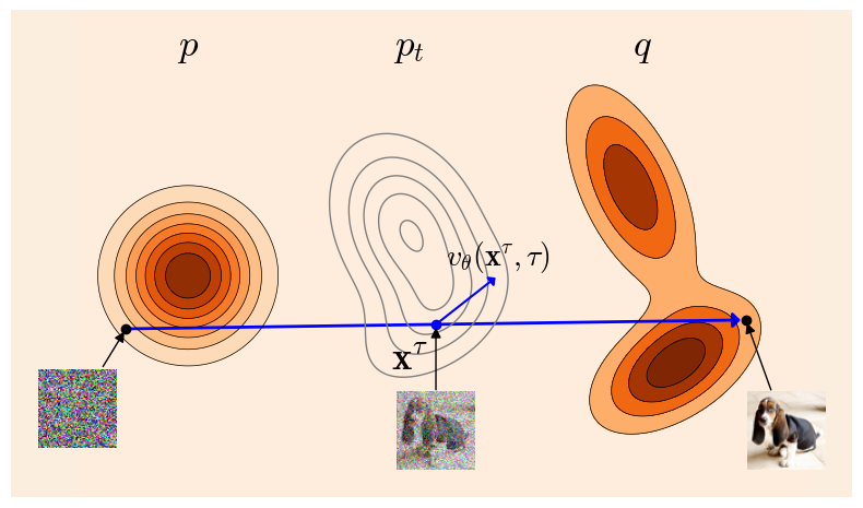
Flow matching은 쉽게 설명하면 perturbed data $\mathbf{x}^\tau$에서 원래 데이터 $\mathbf{x}$ 로 가는 방향을 학습

• 데이터 하나 $\mathbf{x} \in \mathcal{D} \subseteq \mathbb{R}^{d}$, 노이즈 하나 $\bm{\epsilon}\sim\mathcal{N}(\bm{0}_d,I_d)$, 시간 $\tau \in [0, 1]$가 주어졌을 때,
• $\tau$ 시간까지 perturbed된 데이터를 $\mathbf{x}^\tau:=\tau \mathbf{x} + (1-\tau)\bm{\epsilon}$ 라고 하자.

• Flow matching은 $\mathbf{x}^\tau$에서의 velocity $\hat{v}_\theta(\mathbf{x}^\tau, \tau)$를 $\mathbf{x} - \bm{\epsilon}$ 으로 맞춰 준다.

  \[\mathcal{L}_{\text{CFM},\theta}=\mathbb{E}_{\mathbf{x}\sim\mathcal{D},\bm{\epsilon}\sim\mathcal{N},\tau\sim\text{Unif(0,1)}}\left[ \lVert v_\theta(\mathbf{x}^{\tau},\tau) - (\mathbf{x}-\bm{\epsilon}) \rVert_2^2 \right].\]

---

Flow Matching Policy

• Flow matching policy를 위한 objective는 그냥 $o_t$가 condition으로 들어간 것

  \[\mathcal{L}_{\text{CFM},\theta}=\mathbb{E}_{\color{red}{(o_t, a_t)\sim\mathcal{D}},\epsilon\sim\mathcal{N},\tau\sim\text{Unif(0,1)}}\left[ \lVert v_\theta(a_t^{\tau},\tau\color{red}{;o_t}) - (a_t-\epsilon) \rVert_2^2 \right].\]

  
  

• 실제 구현은 각 $(o_t, a_t)\sim \mathcal{D}$마다 $N_{\text{MC}}=8$ 쌍의 $(\epsilon_i,\tau_i)$를 샘플링하여 $\mathcal{L}_{\text{CFM},\theta}$를 근사 (Monte-Carlo estimation)

  \[\hat{\mathcal{L}}_{\text{CFM},\theta}(a_t;o_t)=\frac{1}{N_{\text{MC}}}\sum_{i=1}^{N_{\text{MC}}} \lVert v_\theta(a_t^{\tau_i},\tau_i;o_t) - (a_t-\epsilon_i) \rVert_2^2,\]

  where $a_t^{\tau_i}= \tau_i a_t + (1-\tau_i) \epsilon_i$.

  
  

• 훈련이 완료된 후, 현재 상태 $o_t$에 대한 행동 $a_t$ 샘플링은 다음과 같이 진행

  1. $a_t^{0}=\epsilon \sim \mathcal{N}(0 , I)$
  2. $a_t^{k+1} = a_t^{k} + \frac{1}{M} v_\theta(a_t^{k}, \frac{k}{M};o_t)$ for $k=0, 1, \ldots, M-1$

  (실험에서는 $M=10$ 사용)

---

Proximal Policy Optimization (PPO)

\[ J(\theta)=\mathbb{E}_{\pi_{\theta_{\text{old}}}} \left[ \min\left( \color{blue}{r_t(\theta) \hat{A}_t}, \; \color{green}{\text{clip}\left(r_t(\theta), \, 1-\epsilon, \, 1+\epsilon \right) \hat{A}_t}\right) \right], \]

where $r_t(\theta)=\frac{\pi_\theta(a_t\mid o_t)}{\pi_{\theta_{\text{old}}}(a_t\mid o_t)}$ and $\hat{A}_t$는 advantage estimation인데 주로 GAE를 사용.

---

Objective of FPO

\[ J(\theta)=\mathbb{E}_{\pi_{\theta_{\text{old}}}} \left[ \min\left( \color{red}{r_t^{\text{FPO}}(\theta)} \hat{A}_t, \; \text{clip}\left(\color{red}{\hat{r}_t^{\text{FPO}}(\theta)}, \, 1-\epsilon, \, 1+\epsilon \right) \hat{A}_t\right) \right], \]

where

\[ \hat{r}_t^{\text{FPO}}(\theta):=\exp\left( \hat{\mathcal{L}}_{\text{CFM},\theta_{\text{old}}}(a_t;o_t) - \hat{\mathcal{L}}_{\text{CFM},\theta}(a_t;o_t)\right), \]

where

\[ \hat{\mathcal{L}}_{\text{CFM},\theta}(a_t;o_t)=\frac{1}{N_{\text{MC}}}\sum_{i=1}^{N_{\text{MC}}} \lVert v_\theta(a_t^{\tau_i},\tau_i;o_t) - (a_t-\epsilon_i) \rVert_2^2, \]

where $a_t^{\tau_i}= \tau_i a_t + (1-\tau_i) \epsilon_i$.

---

Experiments

GridWorld

• 환경: $25 \times 25$ 크기의 환경 속에서 에이전트가 위, 아래 각각 2줄 (초록색 영역)에 도착하면 보상을 받음 (sparse reward)
• 왼쪽 그림: 각 셀에서의 FPO 에이전트가 수행한 행동의 평균 벡터
• 중간 그림: FPO 에이전트가 saddle point (별표)에서 생성하는 행동 벡터들.
  • Multi-modal behavior: 생성되는 행동들이 $\tau$가 흐름에 따라 점점 오른쪽 위 행동, 아래 행동으로 나뉨
• 오른쪽 그림: 각 시작 지점에서의 FPO 에이전트의 trajectories.
  • Saddle point에서는 위로 갈 때도 있고, 아래로 갈 때도 있음
  • 각 starting point에서 여러 trajectories들을 만들어 냄 ⇒ Flow matching policy는 diverse action sequence를 모델링할 수 있음

비교: PPO with a Gaussian policy

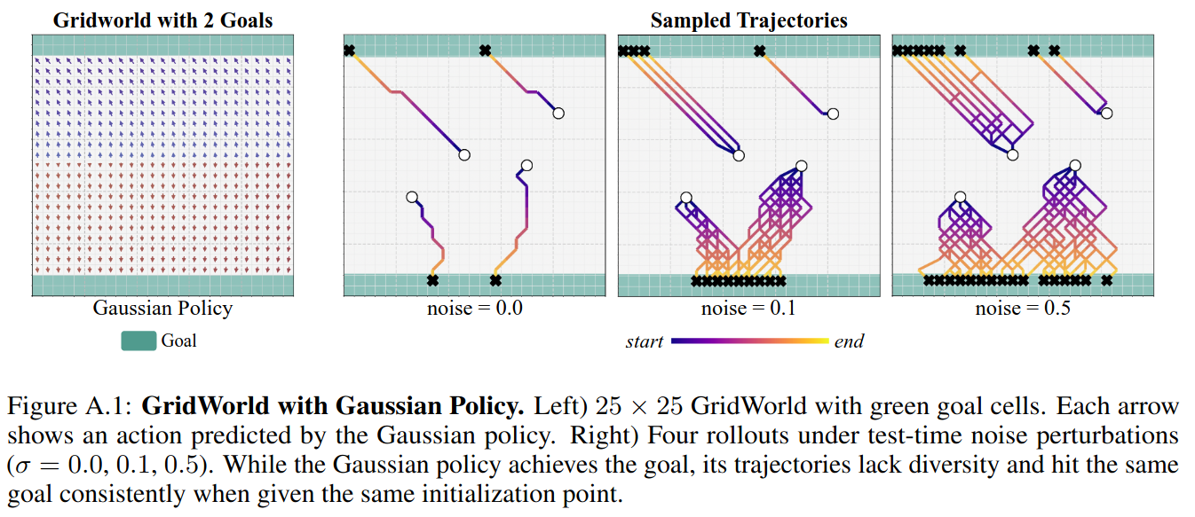
• Trajectories의 diversity가 떨어지고, multi-modal behavior도 나타내지 못한다.

---

Deepmind Control Suite (DMC)

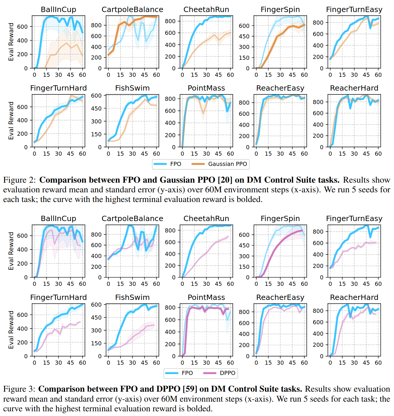
• Figure 2: FPO와 PPO 비교
• Figure 3: FPO와 DPPO 비교
• Policy / velocity networks: MLP(32, 32, 32, 32) / Critic network: MLP(256, 256, 256, 256, 256)

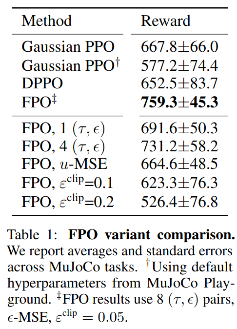
Aggregated performance와 hyperparameter 민감도

---

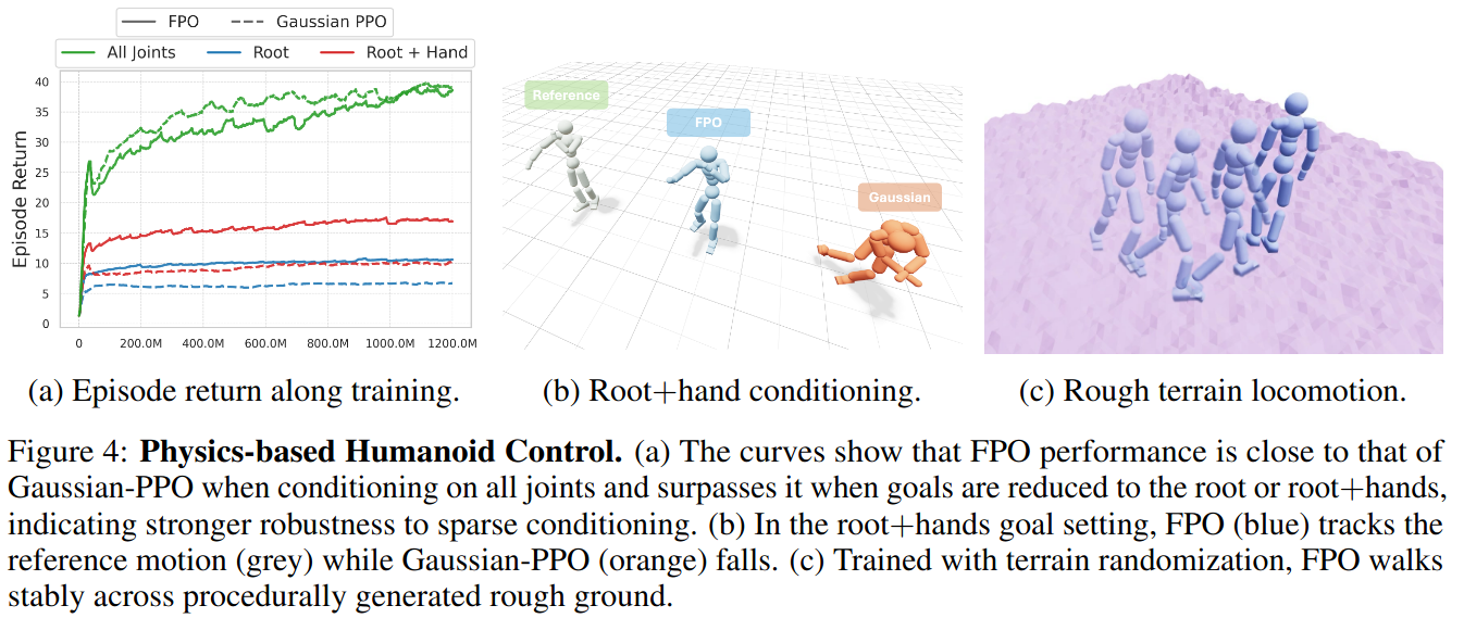
Humanoid Control

Task: Perpetual Humanoid Control (PHC)

• Single policy만으로 주어진 모션들을 imitate하도록 humanoid를 control하는 task.
• AMASS 데이터셋 (11313 motion sequences)을 imitate해야 함
• Policy는 현재 로봇의 proprioceptive observations 뿐만 아니라 reference motion과의 차이를 goal 정보로 전달받음.
  • Reference motion 중 얼마나 많은 관절 정보를 가져올지에 따라 under-conditioned되기도 함
• 훈련시 보상 함수가 자체가 reference motion과의 차이로 정의됨

Results

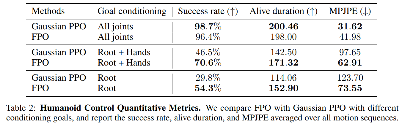
• All joints: Reference motion의 모든 관절에 대한 정보가 goal로 들어왔을 때 성능
• Root: Reference motion의 골반 관절에 대한 정보만 goal로 들어왔을 때 성능 (under conditioning)

---